Learning objectives

In this case study you will be presented to eigen period study of a moored barge from three different perspectives:

1. Eigen period found from stiffness and mass.
2. Eigen period found from direct calculations, applying the AquaSim built-in eigen period analysis tool.
3. Eigen period found from dynamic analysis, where the dynamic response is found, and the natural period is extracted.

Introduction

In this case study, you may apply the AquaSim model Barge.amodel that is associated with this tutorial. Load this in AquaEdit by double-click on the file.

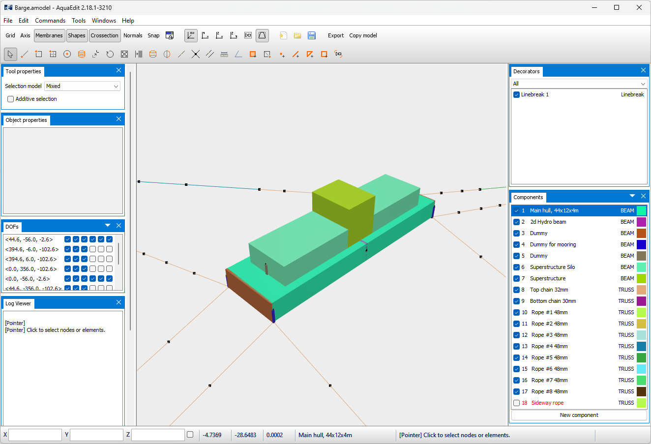
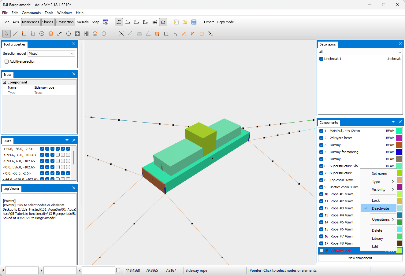
You may notice in the Components window that 18 Sideway rope is deactivated, this should be so until you are notified to activate it.

The main particular of this barge is given in the table below. Both the mass of the barge if self and its associated added mass will contribute to the eigen period.

Length [m]	44.6
Width [m]	12
Draft [m]	2.61
Mass [kg]	1,431,210
Added mass sideways (y-direction) [kg]	858,580

Eigen periods found from stiffness and mass

In this section, the eigen periods are found based on resulting stiffness and mass for the AquaSim analysis. To do so, one has to introduce displacement to the barge. This is done by apply wind on the broad side of the barge (along global y-direction).

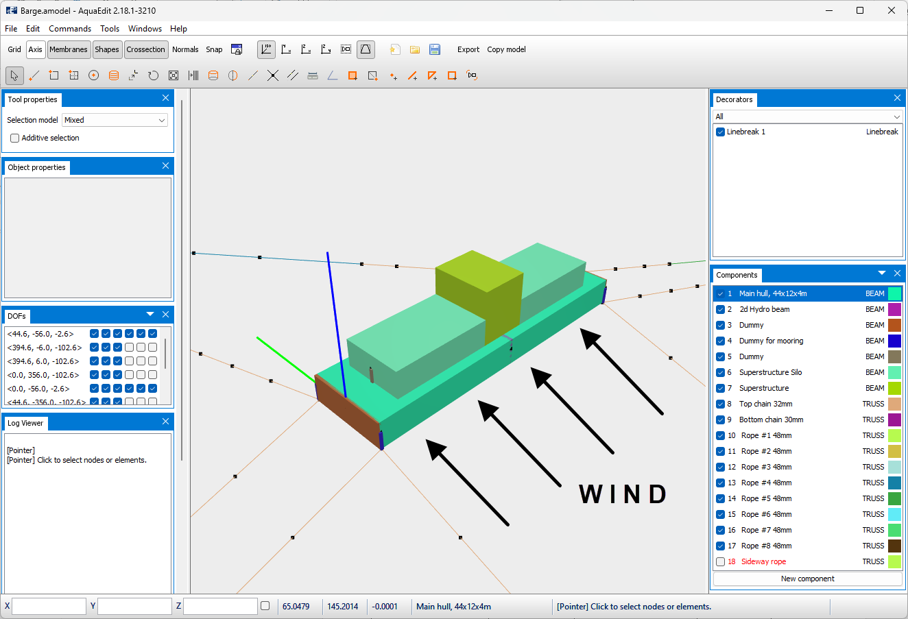
The wind will also induce forces in the mooring line. The eigen period is then found based on the barge displacement and the total horizontal force in the mooring line.

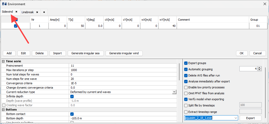
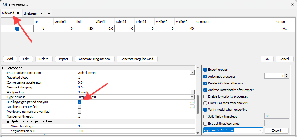
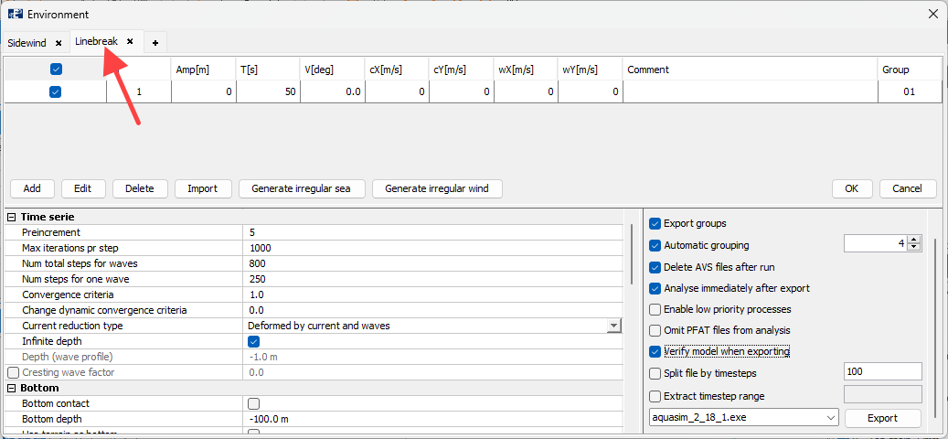
In AquaEdit, select Export and the tab Sidewind. The added mass is dependent on the wave period. The added mass is calculated from T[s] in the input. For this case, this is 50s. As eigen periods vary with both barge mass + added mass, one should be aware of this.

Select Export and start the analysis. Alternatively, you can open the equivalent analysis from the folder Analysis > Barge-Mass-and-Stiffness following this tutorial. Note that if you conduct your own analyses, you will have more files generated than the one following this tutorial. Other files, that is not relevant has been deleted.

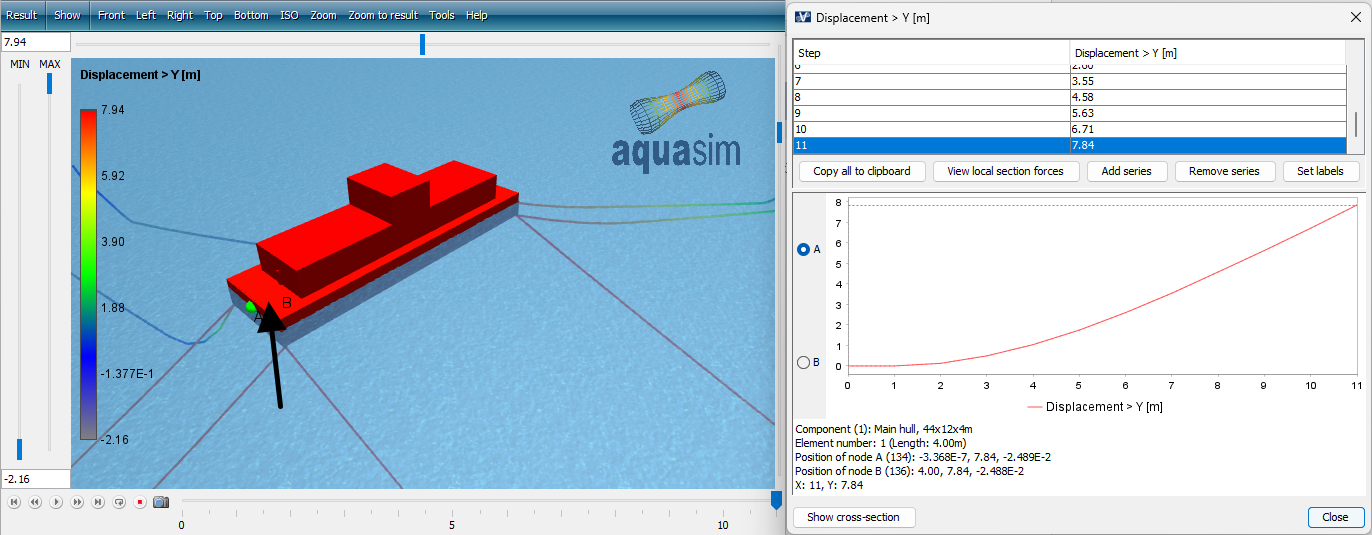
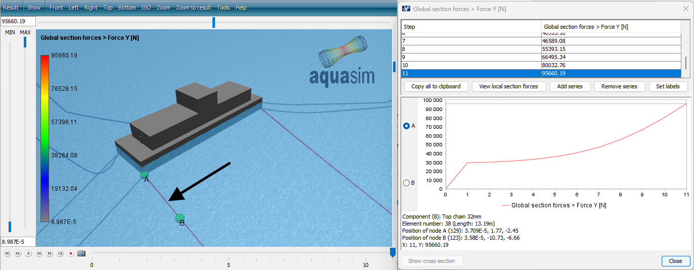
Open the file MassStiffness_01.avz, and plot displacement of the barge in y-direction: Result > Displacement > Displacement Y [m], then click on an element on the barge as shown in the figure below. In AquaSim, wind is applied in incremental steps, meaning that it is linearly increased from 0 to fully developed through the initial static steps in the analysis. This is reflected by an increased displacement of the barge. The displacements from step 1 to 11 are taken out and copied to a table (you may use the attached document Tutorial-Eigenperiods-calculations.xlsx).

Global section force > Force Y [m] is taken out for each mooring line and copied to a table, and the net horizontal force is calculated.

Then tangential stiffness K is found from Hooke’s law (assuming linear relation between force and stiffness):

$${K = \frac{F_y}{r_y}}$$

where \( {F_y} \) is the net horizontal force, and \(r_y\) is the displacement of the barge. The eigen period T is calculated based on:

$${ K - \omega^2 M = 0 \Rightarrow \omega = \sqrt{\frac{K}{M}} \Rightarrow T = 2\pi \sqrt{\frac{M}{K}} }$$

where M is the sum of the barge mass and added mass in y-direction.

The resulting eigen periods for each analysis step are presented in the table below.

F_y (horizontal force y-dir.) [N]	r_y (displacement y-dir.) [m]	K (stiffness) [N/m]	T (eigen period) [s]
2105	0.13	16591	73.8
8242	0.49	17012	72.9
18208	1.03	18300	70.3
31852	1.74	19398	68.3
49052	2.58	20334	66.7
69703	3.52	22032	64.1
93714	4.54	23421	62.1
121004	5.58	26357	58.6
151495	6.65	28397	56.4
185118	7.77	30146	54.8

Eigen periods found from direct calculations

The eigen periods of the barge should now be calculated explicitly from the eigen period analysis tool. The results are then compared with the ones found from mass and stiffness.

In the AquaEdit model, go to the Export menu and select the tab Sidewind. From the Advanced section, select the checkbox Buckling/eigen period analysis

Then select the three dots to the right to enter the control window for eigen period settings. Select input as given in the figure below.

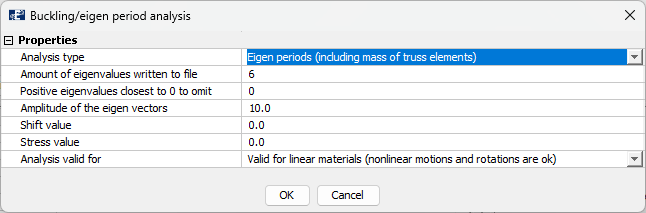
Select OK. Export the model and run the analysis. In this case study, we have named the analysis Direct_. In the analysis-folder, 6 additional files have been generated. The Direct_01eigen1 -6 contain the resulting eigen periods found from the analysis.

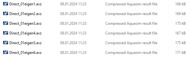
The two succeeding figures (Direct_01eigen1 and Direct_01eigen2 respectively) contain the first and second eigen period of the system. The resulting eigen period is found in Result > Results > Eigenperiod [s].

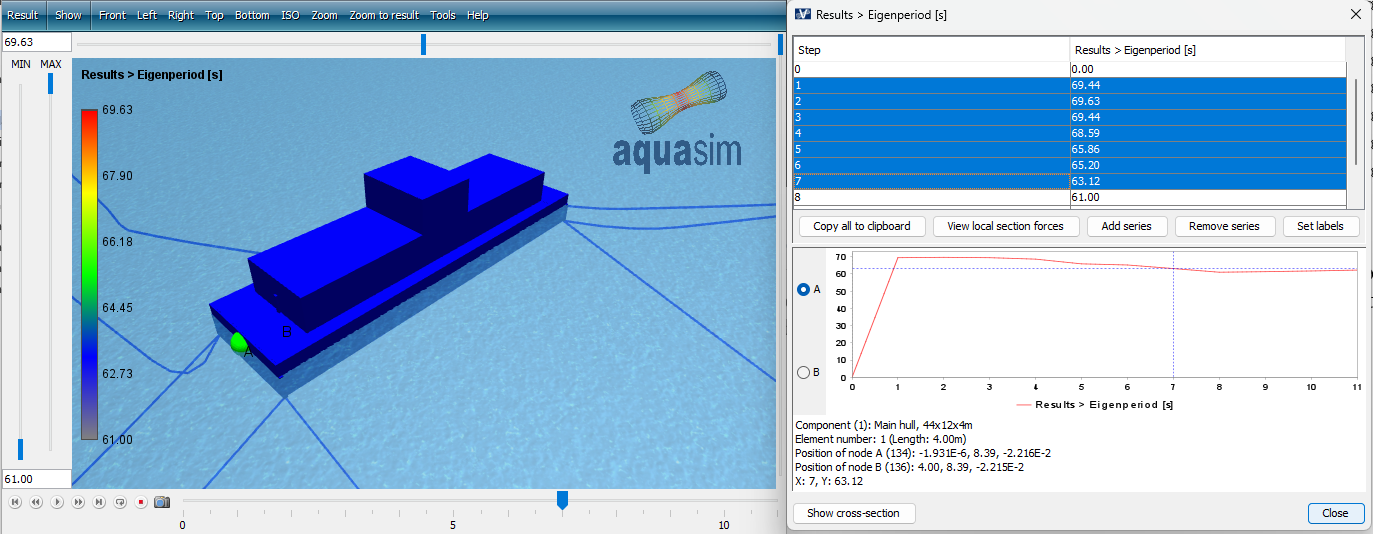
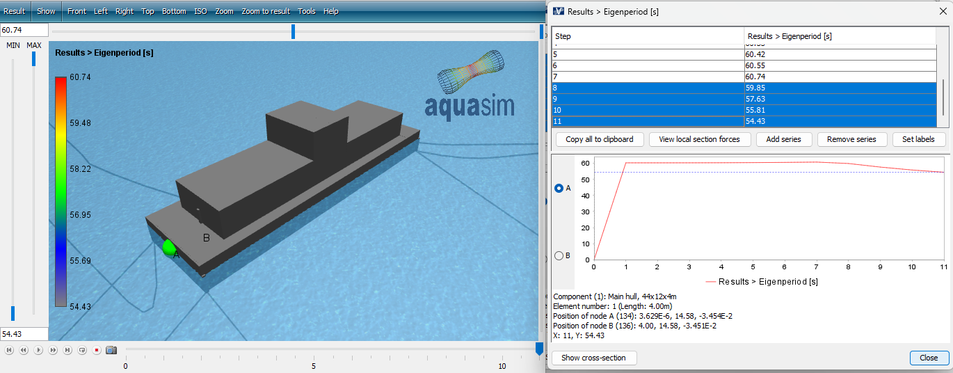
The 7 first steps (out of 11) in Direct_01eigen1 correspond to the first eigen vector for translation along y-axis. Then step no. 8 to 11 in Direct_01eigen2 is the second vector for translation along y-direction. This means that you must consider both files when evaluating eigen periods along y-direction.

Resulting eigen periods from the direct calculations in step no. 1-7 and 8-11 are then compared with the results calculated based on mass and stiffness.

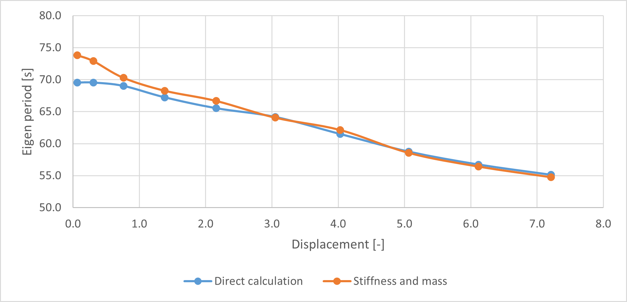
As seen from the graph, results compare well except from in the start. It appears this is due to the stiffness in the direct calculations becomes a bit smaller than the one based on mass and stiffness.

Eigen periods found from dynamic analysis

In this last barge-case-study, an alternative method of studying eigen periods of systems for dynamic problems is presented. Depending on the problem investigated, trusses can be introduced to induce motions to the model.

Return to the AquaEdit model and navigate to the Components window. The last component 18 Sideway rope are two trusses attached to the barge. Activate this component by right click > Deactivate, this will activate the component and the text will go from red to black.

The side ropes are assigned pretension.

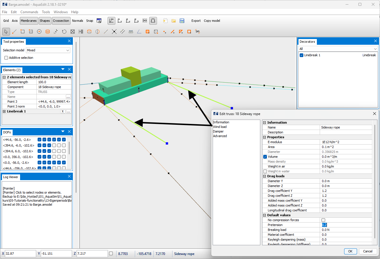
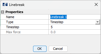
Both side ropes are in addition assigned Linebreak.

The pretension will cause the barge to be pushed to the side. This is equivalent as being conducted in model basin tests. This means that this is a good analysis to carry out for cases where model basin testing is compared with analyses.

Return to the Export menu and select the tab Linebreak. Export the model and run an analysis.

We named the analysis Dynamic_. Load the associated avz-file in AquaView and plot displacement in y-direction: Result > Displacement > Displacement Y [m]*.

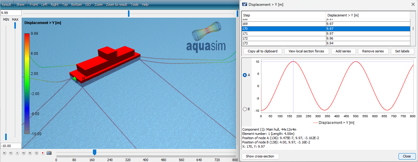
By measuring the time difference between the peaks, one finds that the period of this resonant response is approximate 66 seconds. This compares fairly well with the explicit analysis.