AquaEdit

Let as investigate the opportunities that comes with drift coefficients. More in-depth theory for drift forces and drift coefficient can be found in the textbook Sea loads on ships and offshore structures by Faltinsen (1990).

In AquaEdit one may introduce drift forces to a node in a similar way as RAO on loads and displacements to a node. Instead for displacement/force/moment-amplitudes drift coefficients are introduced.

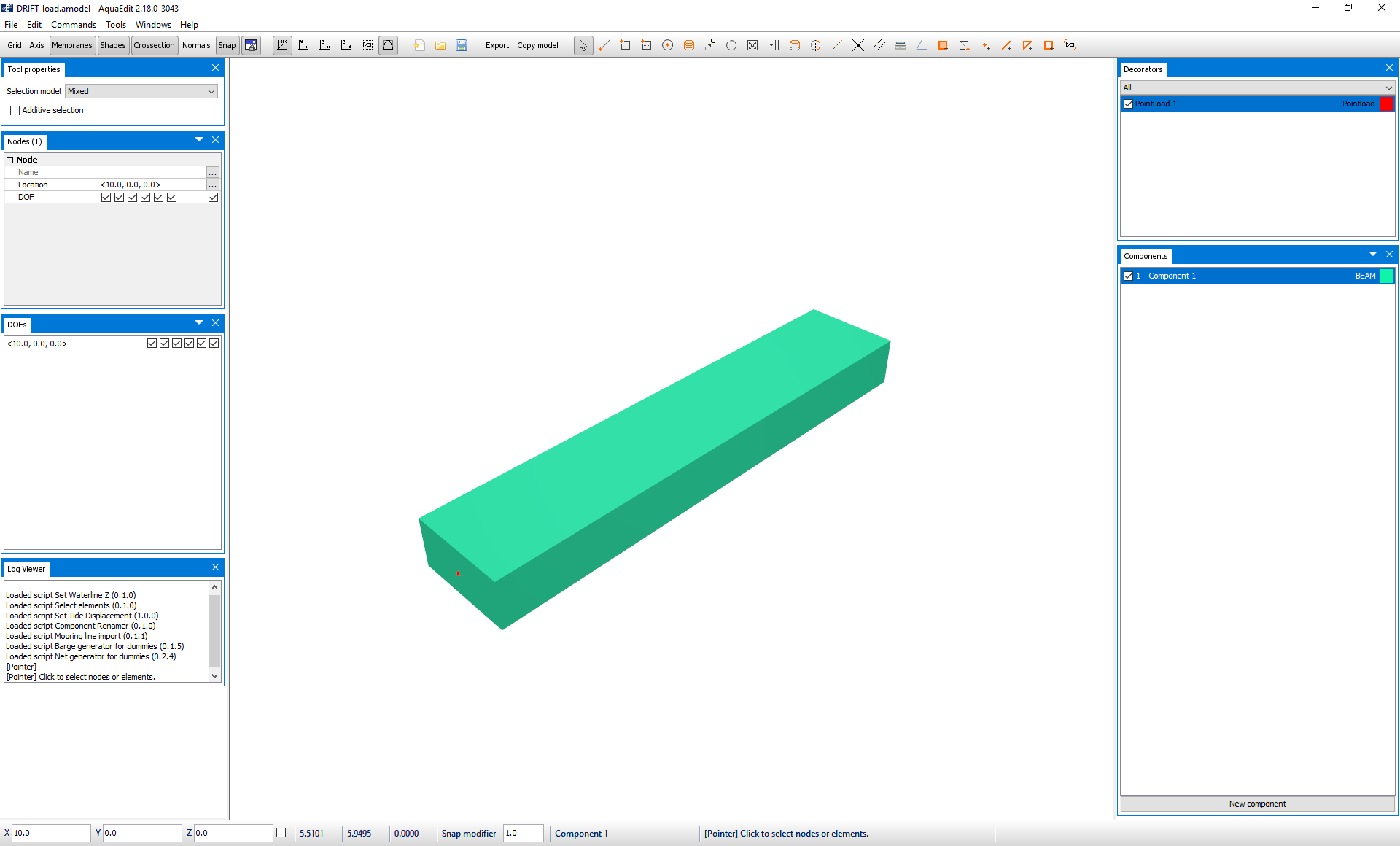
Load the AquaEdit model DRIFT-load.amodel. This beam model is equivalent as for the load-RAO case. Where one node is fixed, and the other is assigned a Pointload. Double click on the prepared node decorator Pointload 1 to enter the Edit Pointload-window.

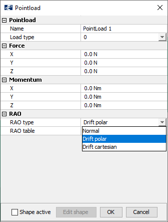
In the section, RAO type, we see that AquaSim provides the options to apply Drift in two ways:

• Drift polar: the drift force is in the direction of the wave and is equal for all direction. This is good to use for circular objects.
• Drift cartesian: When applying drift cartesian, the drift force is given in cartesian coordinates, where headings in different directions may give different responses. The response does not need to be only in the direction of the wave. It is linearly interpolated between angles. As was demonstrated in the previous case.

We select Drift Polar. In the RAO table section, select the drop-down menu and select the table RAO-Drift-polar. Enter the table through selecting the three dots to the right.

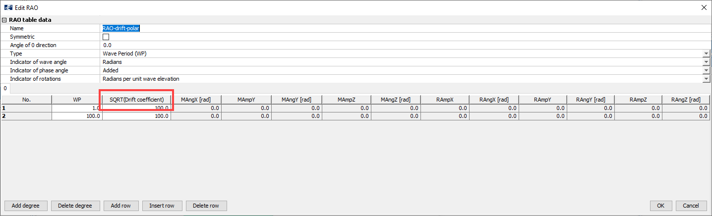
Remember the equation presented in the introducing chapter of this tutorial. It is \(\sqrt{T}\) that is the input to AquaSim. In the above figure this is called SQRT(Drift coefficient).

The other sections along here are deactivated as they are of no relevance. A drift coefficient of 100 is applied for wave period equal to 1 and 100. We are satisfied with the parameters in the table and Exit the windows.

Analysis

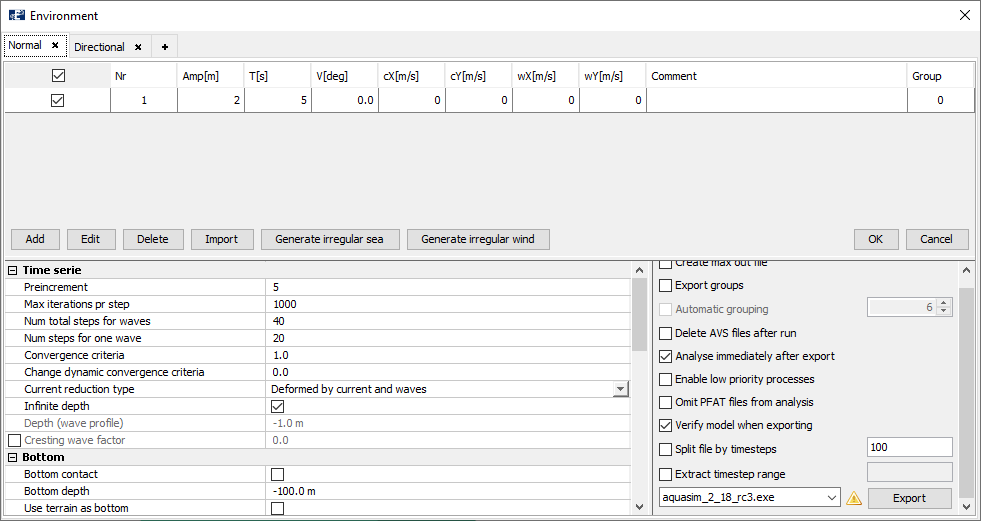
The basis for the analysis is the same as the previous cases. In AquaEdit select Export to enter the Environment-window. Use the Normal-tab where a load condition is prepared.

Export the analysis, save it a suitable place, and Start the analysis.

AquaView

Load the result-file in AquaView through selecting Open in the Analyse window. The below figure shows the axial force in the beam plotted.

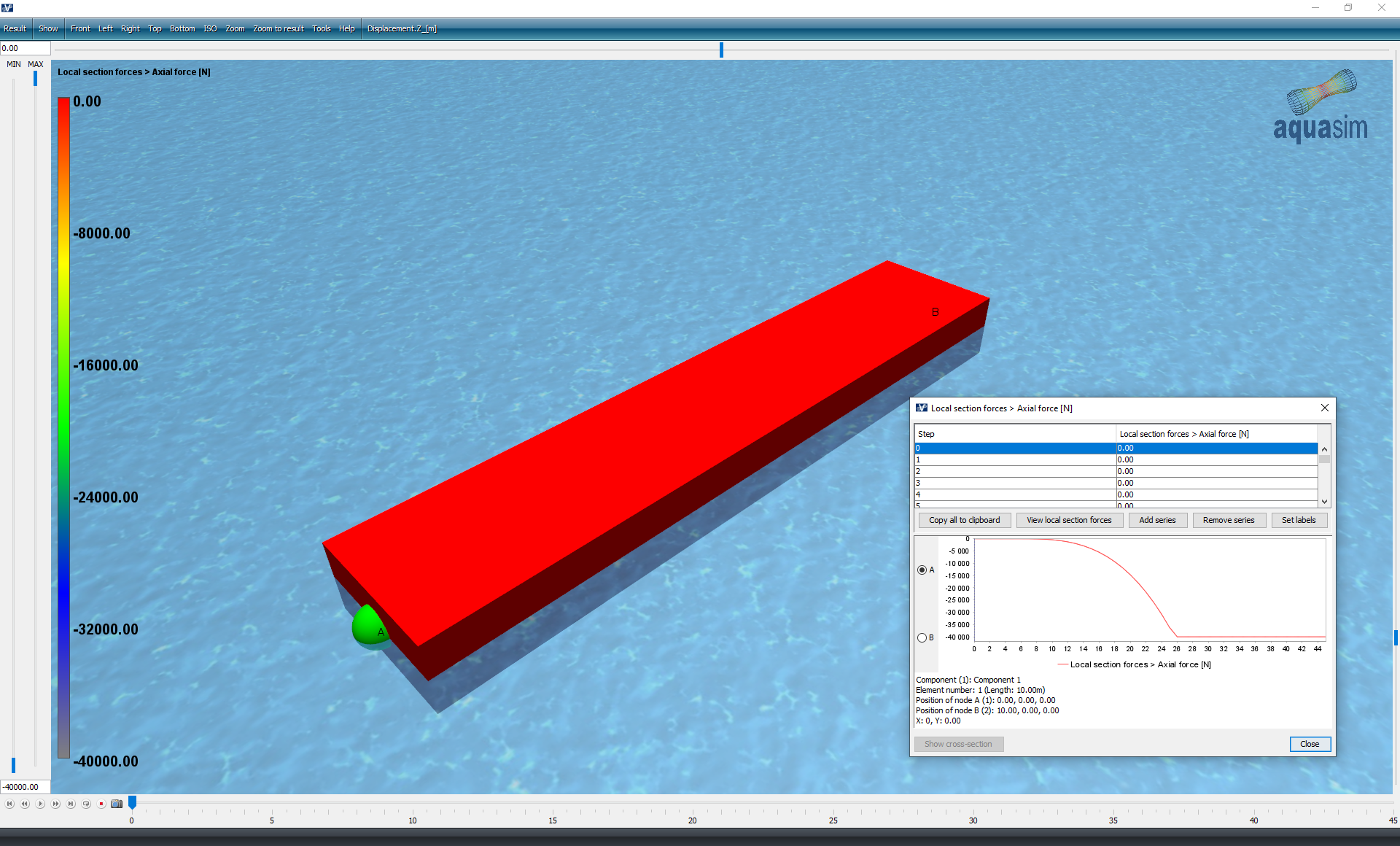
When the wave angle is 0 degrees, and the drift coefficient is 100 times 100, the drift coefficient is multiplied with the wave height squared and multiplied with 2. As given in the presented equation. This means the force will be a sinusoidal force with an amplitude of 80000 newton. AquaSim combine values at the time and a quarter wave cycle at the mean zero crossing period to filter out the sum frequency effect. This means it then fits that the force equals to 40000 newtons for the analysed case.

Irregular wave spectra

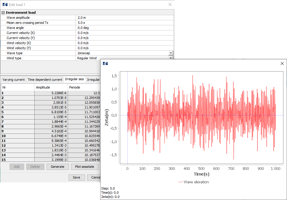
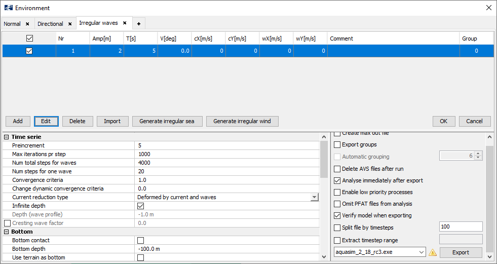
A case applying irregular wave spectra can be applied. Go back to your AquaEdit model and select Export. In the Environment window, go to the tab that is named Irregular waves.

The same wave amplitude and wave period is applied as the basis for a wave spectrum. When wave spectra are applied the section for Amp[m] and T[s] is greyed out. Click on the load condition line and select Edit. A JONSWAP wave spectrum is generated, and you can plot the spectrum through selecting Plot seastate.

The wave spectrum is generated with 200 wave components. In the Time serie section, we have Num total steps for waves = 4000 and Num steps for one wave = 20.

Then run a new analysis. When it is finished open the result-file in AquaView and plot the axial forces: Result > Local section forces > Axial force [N].

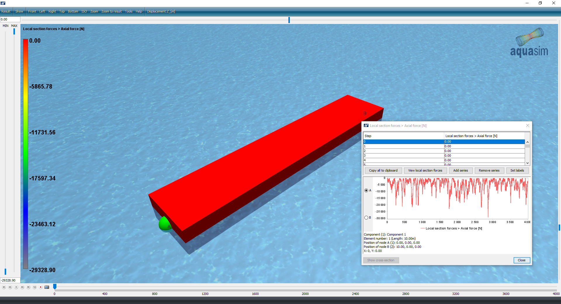
For irregular waves, the drift forces will rather be a slowly varying force rather than a constant force. This fits well with the figure above.