“Flexible tarp” load formulation stems from the recognition seen in tank testing, e.g. (Roaldsnes, 2020) that much of waves passed though the tarpaulin with little influence on the waves by the tarpaulin. It describes forces, added mass and damping on soft and flexible textiles can be modeled to resemble this. Characteristic for such structures, as lice skirts, is that a large part of the wave passes through more or less undisturbed, rather than scattering the waves as rigid bodies would.

The flexible tarp formulation is suitable for structures that are highly compliant, where they move with the water. This is called damping-dominated behavior where the structure’s response is mainly determined by how much the structure resist motion through damping.

Theoretical basis

As mentioned, wave excitation loads are composed of Froude-Kriloff and diffraction forces. Unlike rigid bodies, flexible textiles do not produce significant scattered waves, so the diffraction term is neglected. The “Flexible tarp” formulation is hence described only by the undisturbed Froude-Kriloff pressure. Following e.g. (Faltinsen, 1990) this pressure is described as:

$${ p(x, z, t) = \rho g \zeta_A e^{kz} \sin(kx - \omega t) }$$ Equation 1

where

• \(\rho\) is the density of seawater,
• \( g \) is the acceleration of gravity
• \( \zeta_A \) is the wave amplitude,
• \(z\) is vertical location,
• \(k\) is wave number,
• \(x\) is location along x-direction,
• \(\omega \) is wave frequency,
• \(t\) is time.

Presenting the horizontal fluid particle velocity due to waves: $${ u(x, z, t) = \omega \zeta_A e^{kz} \sin(kx - \omega t) }$$ Equation 2

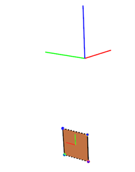
Now, consider a simple membrane panel in the yz-plane, as shown in Figure 6. This panel as an area A.

Introduce this panel area to the equation for pressure (Equation 1) we get the Froude-Kriloff force:

$${ F(x, z, t) = A , \rho g \zeta_A e^{kz} \sin(kx - \omega t) }$$

Equation 3

This is simply the undisturbed wave pressure field integrated over the structure’s wetted surface.

Analysis

Froude-Kriloff pressure

The aim of this section is to present how the Froude-Kriloff pressure is calculated in AquaSim by establishing a simple model and compare analysis with analytical results. Consider a membrane panel with an area of \(A = 4\text{m}^2\). The panel is restrained with truss elements in each corner; this is illustrated in Figure 7.

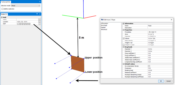
Each node on the panel is free to move along x-direction. Wave loads on the panel will be distributed as axial forces to the trusses. An analysis is carried out with wave data as presented in Table 2.

Table 2 Wave data applied to analysis

Parameter		Value
\( \text{Wave amplitude [m]} \)	\( \zeta_A \)	\( 1 \)
\( \text{Density [kg/m}^3\text{]} \)	\( \rho \)	\( 1025 \)
\( \text{Period [s]} \)	\( t \)	\( 100 \)
\( \text{Wave frequency [1/s]} \)	\( \omega \)	\( 6.28E-02\)
\( \text{Wave number [1/m]} \)	\( k \)	\( 4.02E-04 \)
\( \text{Position, z-upper [m]} \)	\( z_{\text{upper}} \)	\( -5 \)
\( \text{Position, z-lower [m]} \)	\( z_{\text{lower}} \)	\( -7 \)
\( \text{ekz-upper}\)	\( e^{kz_{\text{upper}}} \)	\( 0.99799 \)
\( \text{ekz-lower}\)	\( e^{kz_{\text{lower}}} \)	\( 0.997187 \)
\( \text{Pressure upper [N/m}^2\text{]} \)	\( p_{\text{upper}} \)	\( 10035.04 \)
\( \text{Pressure lower [N/m}^2\text{]} \)	\( p_{\text{lower}} \)	\( 10026.96 \)

Since the panel area is 4m2, the forces in each truss should correspond to the pressure presented in Table 2. Figure 8 and Figure 9 show the resulting axial force from AquaSim in one of the upper trusses, and one of the lower. The upper truss takes up approximately 10034 N and the lower 10028 N. This corresponds well with the calculations in Table 2.

Horizontal panel response

The concept behind this section is to conduct an analysis to show that, in absence of any other external forces than the Froude-Kriloff pressure, the panel’s motion should follow the wave particle motion of the surrounding fluid. This occurs when the Froude-Kriloff pressure is applied to the panel in the direction of the wave. To achieve this behavior, damping force \(F_D\) is introduced such that the resulting horizontal velocity of the panel u will match the wave particle velocity when subject to Froude-Kriloff pressure:

$${ F_D \cdot u = F }$$

where F is the Froude-Kriloff force. We then insert the expression for Froude-Kriloff force from Equation 3, and the horizontal fluid particle velocity from Equation 2, and get:

$${ F_D = \frac{F}{u} = \frac{A \cdot \rho g \zeta_A e^{kz} \sin(kx - \omega t)} {\omega \zeta_A e^{kz} \sin(kx - \omega t)} = \frac{A \cdot \rho g}{\omega} }$$

Equation 4

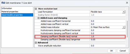
This means that if the damping term ρg/ω is introduced to the membrane panel per m2, the response should follow the wave particle motion. In AquaSim, this corresponds to having the parameter “Damping coefficient (flexible tarp)” set to 1.0, see Figure 10.

The damping force introduced to the membrane panel becomes:

$${ F_D = \frac{\text{Damping coefficient (flexible tarp)} \cdot A \rho g}{\omega}}$$

Equation 5

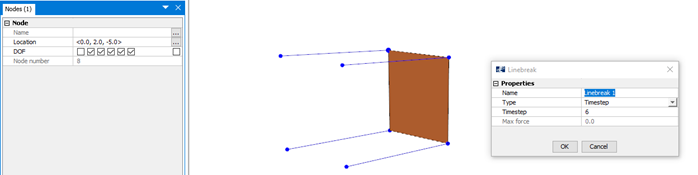
Go back to your model in AquaEdit. To enable the panel to move with the fluid particle motion, the trusses must be removed. They should not be deleted from the model, as this will lead to equilibrium not being found. We need the trusses so that the Froude-Kriloff pressure can be induced on the panel. Instead, we remove the trusses in the first dynamic step in the analysis by applying the Linebreake-function, see Figure 11. The panel is still free to move only in x-direction.

Analysis is run with the same wave parameters as presented in Table 2. The horizontal displacement of the panel is presented in Figure 12 and Figure 13. The results indicate that the panel follows the fluid particle motion as it has a sinusoidal response. Which is consistent with linear wave theory applied.

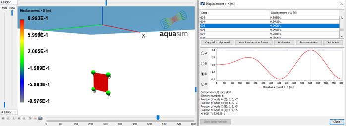
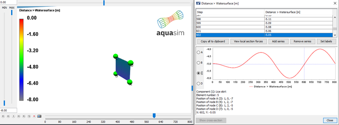
When we consider distance to the water surface, for the same timestep as in Figure 12 and Figure 13, we see that the displacement is approximately 90 degrees after the wave elevation. This phase-relation is in line with the circular motion of the fluid particles.

Horizontal displacement ξ of the panel is found by integrating the horizontal fluid particle velocity over time:

$${ \xi(x, z, t) = \int u \ dt }$$

where the maximum displacement is found as:

$${ \xi_{\text{MAX}}(x, z, t) = \zeta_A \cdot e^{kz} }$$

From Table 2 we know \(ζ_A=1.0m\) and the upper node is located at \(z_{upper}=-5m\) and the lower \(z_{lower}\)=-7m. This results in the displacement as presented in Table 3. Comparing AquaSim and analytical, the results fit well.

Table 3 Displacement of panel, analytical vs AquaSim

	Analytical	AquaSim
Displacement X, upper	0.9980	0.9981
Displacement X, lower	0.9972	0.997

Vertical panel response

In the vertical direction, the panel motion is in phase with both the pressure field and the wave surface elevation. This means that the relationship between vertical fluid motion and resulting panel response can be expressed in terms of an equivalent stiffness term. However, a stiffness term requires a defined reference position. So, it will be advantageous to handle the vertical direction by also using damping term as in Equation 5. The following algorithm is therefore applied to the vertical direction:

• A force equivalent to the Froude-Kriloff force is applied but shifted 90 degrees ahead of the Froude-Kriloff pressure in phase.
• A damping force is then applied.

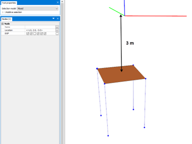
Consider the same panel, only now rotated 90 degrees, as illustrated in Figure 15. The panel is free to displace in z-direction. The panel is located at a depth of 3 meters.

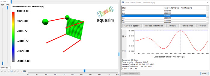
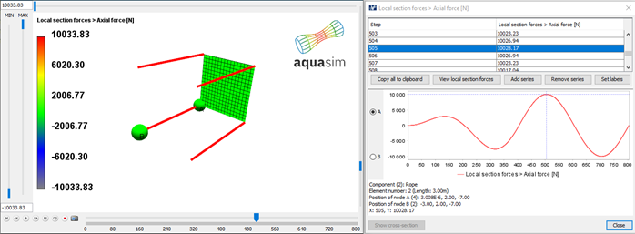
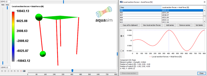
An analysis with the same parameters as presented in Table 2 is run. This will result in forces as shown in Figure 16.

Conducting the same analysis, now applying the function Linebreake to observe the vertical motion of the panel. The resulting displacement in z-direction is presented in Figure 17.

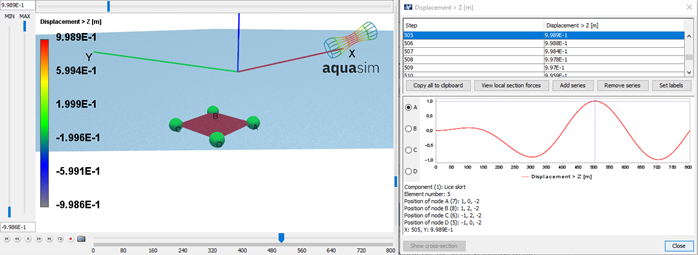
Figure 18 presents how the Froude-Kriloff dynamic wave pressure is in phase with the vertical displacement in Figure 17.

By comparing Figure 18 and Figure 16 it is observed that the axial force in the truss is 90 degrees ahead of the wave elevation. This indicates that when the response is governed by damping term, the vertical motion (as shown in Figure 17 and Figure 18) is in phase with the Froude-Kriloff pressure.

Damping coefficient (flexible tarp)

As lice skirts are highly flexible, their behavior can be characterized as damping-dominated, where the response amplitude is mainly determined by how much the lice skirt resist motion through damping. In AquaSim, the two parameters controlling the response of the lice skirt are shown in Figure 19

These coefficients are implemented to AquaSim as follows:

• Damping coefficient (flexible tarp) normal: Regulates the damping force in direction normal to the membrane panel as described in Equation 5, and reproduced below: $${ F_{D(\mathrm{normal})} = \frac{Damping\ coefficient(flexible\ tarp)\ \cdot A \rho g}{\omega} }$$
• Damping coefficient (flexible tarp) tangential: Regulated the damping force in direction tangential to the membrane panel. The same damping as in the normal direction is applied here and scaled with the coefficient. Meaning: $${F_{D(\mathrm{tangential})} = Damping\ coefficient\ (flexible\ tarp)\ \text{tangential to panels}\ \cdot\ F_{D(\mathrm{normal})}}$$