Validity

The analytical solution for calculating the wave excitation pressure and forces, described in (Maccamy & Fuchs, 1954), is based on linear potential flow theory and assumes an infinitely long vertically oriented circular cylinder with a fixed radius. Meaning that infinite water depth is assumed (deep-water waves). Therefore, care should be taken, when using this load formulation for analysing anything other than what is assumed for this load formulation.

Furthermore, if you are using the “MacCamy-Fuchs” load formulation to analyse a vertical cylinder with fixed radius and finite length, one should be careful with respect to evaluating which wave periods that one might consider valid for the structure under consideration.

A rule of thumb will be to assume that the load formulation will provide sufficiently accurate results for a wave period (T) corresponding to a wavelength (λ) of twice the length of the cylinder (L) or less, i.e. \( \lambda \leq 2L \), where \( \lambda = \frac{g}{2\pi} T^2 \) for deep-water waves. For example, given a cylinder with fixed radius and a length L=110m, this load formulation should at least be valid for wave lengths \(\lambda \leq 220 \text{m} \), corresponding to wave periods of \(T \leq 11.9 \text{s} \) assuming deep-water waves.

In general care should be taken when analyzing structures with the “MacCamy-Fuchs” load formulation where diffraction is of importance, meaning for wavelengths shorter than 5 times the diameter of the cylinder (D), i.e. \(\lambda < 5 \cdot D \), as well as when the wavelength is greater than twice the length of the cylinder, i.e. \(\lambda \geq 2L \). Typically, this corresponds to short cylinders with large diameters.

Total wave excitation pressure

The total wave excitation pressure using the “MacCamy-Fuchs” load formulation in AquaSim is calculated as described by Equation 1 - Equation 6. Abbreviations are given in Table 1. For more details, see (Maccamy & Fuchs, 1954) and (Aquastructures AS, 2024a).

Table 1 Abbreviations for parameters in the “MacCamy-Fuchs” load formulation.

Abbreviation	Description	Unit
ρ	Density of water, 1025	kg/m³
g	Gravitational acceleration, 9.81	m/s²
ζ	Wave amplitude	m
k	Wave number	1/m
z	Vertical position, 0 means still water level. Positive upwards.	m
h	Depth of sea bottom	m
i	Complex unit (0,1)	–
Bn	Coefficient, see Equation 2	–
Hn	Hankel function, first kind	–
J′n	Bessel function, derivative	–
εn	ε0 = 1, else 2	–
ω	Wave frequency	rad/s
t	Time	s

The diffraction pressure from “MacCamy-Fuchs” is calculated as: $${p_{MF} = \rho g \zeta \dfrac{\cosh k(z+h)}{\cosh kh} \sum_{n=0}^{\infty} i\left[B_n {H_n}^1(kr)\right] \cos n\theta , e^{-i\omega t}}$$ Equation 1

Where:

$${ B_n = -\varepsilon_n i^n \dfrac{J_n^{\cdot}(kr)}{H_n^{(1)^{\cdot}}(kr)} }$$

Equation 2

The Frode-Kriloff pressure in a regular sea with airy waves, from the incident wave is found as:

$${ p_{FC} = \rho g \zeta \dfrac{\cosh k(z+h)}{\cosh kh} \sin(\omega t - kx) }$$

Equation 3

If irregular waves are considered, the pressure from the diffracted wave field on the surface of the structure is found as:

$${ p_{MF} = \sum_{m=1}^{N} \rho g \zeta_m \dfrac{\cosh k_m(z+h)}{\cosh k_m h} \sum_{n=0}^{\infty} i\left[B_n {H_n}^{1}(kr)\right] \cos n\theta \space e^{-i\omega t + \varepsilon_n} }$$

Equation 4

While the Frode-Kriloff pressure for an irregular sea is found as:

$${ p_{FC} = \sum_{n=1}^{N} \rho g \zeta_n \dfrac{\cosh k_n(z+h)}{\cosh k_n h} \sin(\omega_n t - k_n x + \varepsilon_n) }$$

Equation 5

The total pressure at a given point is then found as:

$${ p = p_{FC} + p_{MF} }$$

Equation 6

Since the “MacCamy-Fuchs” theory for diffracted waves is only valid for vertical cylinders, the pressure from the diffracted wave field \( p_{MF} \) is multiplied with the vertical projection of the area.

Added mass and hydrodynamic damping

Both the added mass and hydrodynamic damping are calculated in a simplified manner when using the “MacCamy-Fuchs” load formulation and relates these parameters to the geometry and the volume of the structure and are therefore also frequency independent, using this load formulation. The reason being that the “MacCamy-Fuchs” load formulation only analytically solves the “diffraction problem” and not the “radiation problem”. This methodology is identical to the methodology for calculating the dynamic inner fluid mass, and detailed descriptions and figures can be found in (Aquastructures AS, 2025c).

Vertically oriented panels

For vertically oriented panels with otherwise arbitrary orientation, the horizontal (normal) added mass and hydrodynamic damping per m2 are calculated as follows:

$${ \text{Added mass per m}^2 \text{, horizontal} = R \cdot C_{Amass_{hor}} \cdot \rho \cdot \hat{r}_{hor} \cdot \hat{n}_{hor} }$$ Equation 7

$${ \text{Hydrodynamic damping per m}^2 \text{, horizontal} = R \cdot C_{Hdamp,hor} \cdot \rho \cdot \hat{r}_{hor} \cdot \hat{n}_{hor} }$$ Equation 8

Here R is the distance from the panel to the geometric centerline of the 2D volume of the structure at the vertical position of the panel as seen in Figure 1. \( C_{Amass_{hor}} \) and \( C_{Hdamp,hor} \) are the horizontal coefficients for added mass and hydrodynamic damping, as highlighted in yellow in Figure 2. The vectors \( \hat{r}_{hor} \) and \( \hat{n}_{hor} \) are the normalized horizontal position vector of the panel and the normalized horizontal normal vector of the panel respectively. Furthermore, ρ is the density of seawater (1025 kg/m^3).

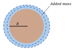
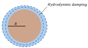
Figure 1 Illustration of the distance R.

Horizontally oriented panels

For horizontally oriented panels with otherwise arbitrary orientation, the vertical (normal) added mass and hydrodynamic damping per \( m^2 \) are calculated as follows:

$${ \text{Added mass per m}^2 \text{, vertical} = z_{pos} \cdot C_{Amass_{vert}} \cdot \rho }$$ Equation 9

$${ \text{Hydrodynamic damping per m}^2 \text{, vertical} = z_{pos} \cdot C_{Hdamp_{vert}} \cdot \rho }$$

Equation 10

\( C_{Amass_{vert}} \) and \( C_{Hdamp_{vert}} \) are the vertical coefficients for added mass and hydrodynamic damping, as highlighted in green in Figure 2.

Arbitrary oriented panels

For arbitrary oriented panels the added mass and hydrodynamic damping per m2, acting normally on the panel, are calculated as follows:

$${ \text{Added mass per m}^2 = \rho \left( z_{pos} \cdot \sqrt{n_z^2} \cdot C_{Amass_{vert}} + R \cdot \hat{r}_{hor} \cdot \hat{n}_{hor} \space \sqrt{1-n_z^2} \cdot C_{Amass_{hor}} \right) }$$

Equation 11

$${ \text{Hydrodynamic damping per m}^2 = \rho \left( z_{pos} \cdot \sqrt{n_z^2} \cdot C_{Hdamp_{vert}} + R \cdot \hat{r}_{hor} \cdot \hat{n}_{hor} \cdot \sqrt{1-n_z^2} \cdot C_{Hdamp_{hor}} \right) }$$

Equation 12

Here \( \sqrt{n_z^2} \) and \( \sqrt{1-n_z^2} \) are the absolute values of the vertical and horizontal component of the unit normal vector of the panel, respectively.

Other notes on added mass and hydrodynamic damping

Because of this formulation, the total vertical and total horizontal added mass and hydrodynamic damping are directly proportional to the total 3D volume of the structure, as long as the structure either consists strictly of horizontal and vertical panels (e.g. cylinders, box shapes etc.) or has radial symmetry (e.g. spheres, half spheres etc.).

Note 1: The exact same methodology is applied for calculating the added mass and hydrodynamic damping when using the load formulation “Flexible tarp”.

Note 2: The added mass coefficients \( C_{Amass_{hor}} \) and \( C_{Amass_{vert}} \) are unitless. The hydrodynamic damping coefficients \( C_{Hdamp_{hor}} \) and \( C_{Hdamp_{vert}} \) have unit [1/s], when using the “Flexible tarp” and “MacCamy-Fuchs” load formulations, but are unitless when using the “Numerical diffraction” load formulation.

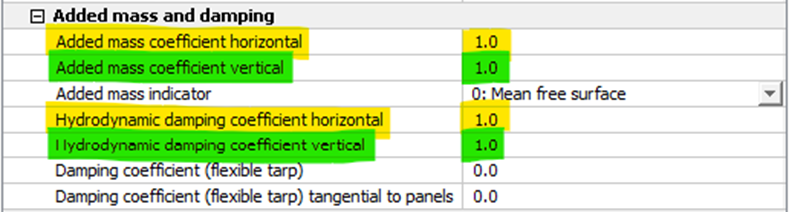
Figure 2 Added mass and hydrodynamic damping coefficients.