Discretization

One important aspect was not considered when the model was established in AquaEdit: discretization. In this section, you are going to see the effect of discretization of the model on analysis results. Go back to your model in AquaEdit or chose the premade model from Documents\AquaSim\Demoes\CaseStudy_01\CaseStudy01.amodel.

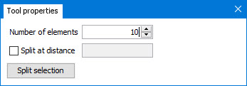
The premade model is loaded in AquaEdit by double click on the file. You should divide the element into smaller entities. From the intents in the Toolbar menu, select Split line . The Tool properties window is activated in the left docking area, with settings for splitting of elements. In the row Number of elements, type 10 and press ENTER (alternatively select the arrow until you get 10).

Move the mouse pointer to the 3D view until it is situated above the beam element, then left click.

Your beam should now consist of 10 elements.

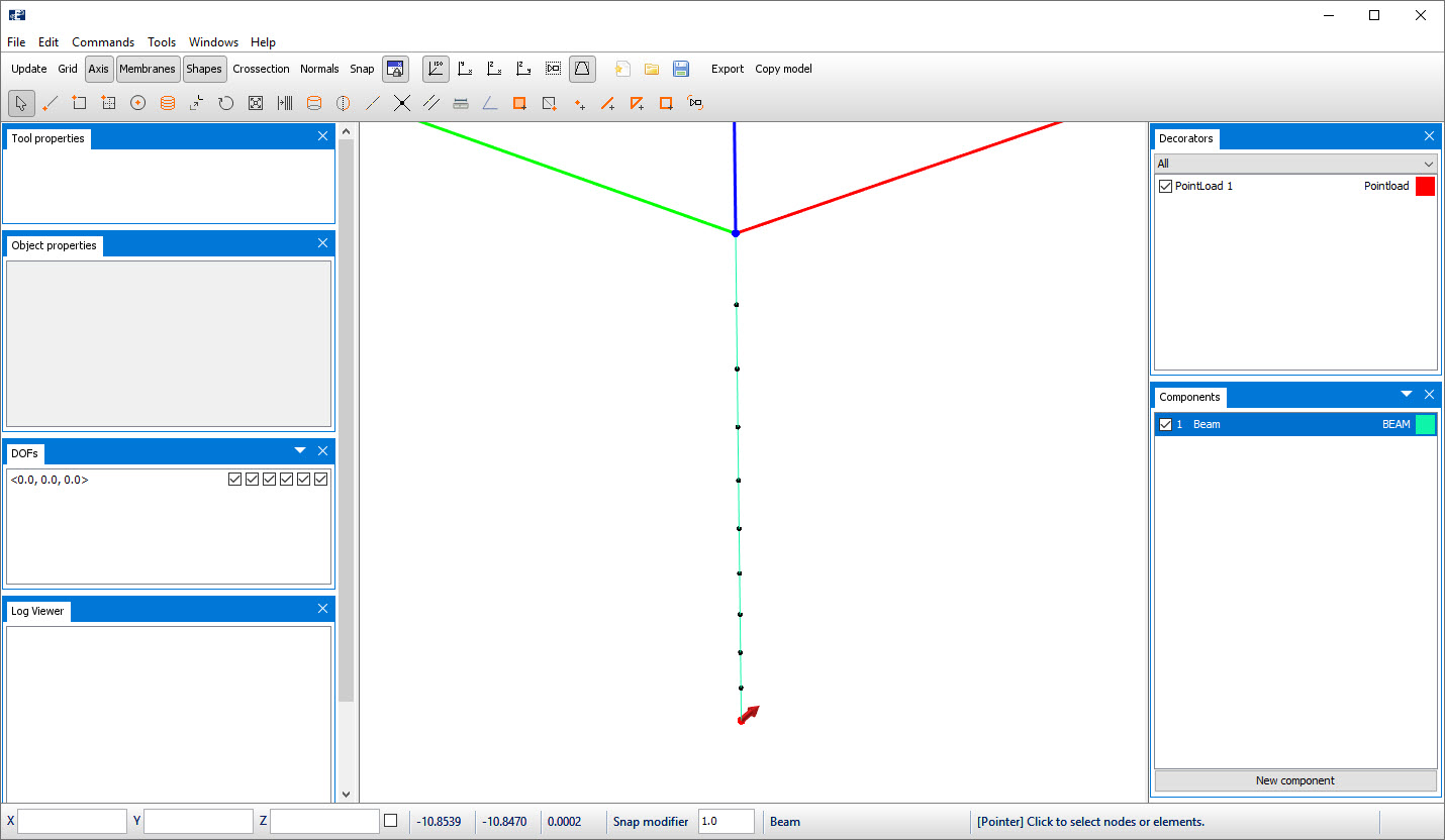All the elements that constitute your beam shear the same properties because they are grouped within the same component Beam.

Visual Cross Section

Until now, your beam is just presented as a straight line in the 3D view. From Properties of Beam component. in this case study, you remember the beam was assigned a visual cross section. To turn on the display of the cross section, select from the Toolbar. Then, zoom into the beam by Scrolling upwards.

Enter Environment Window

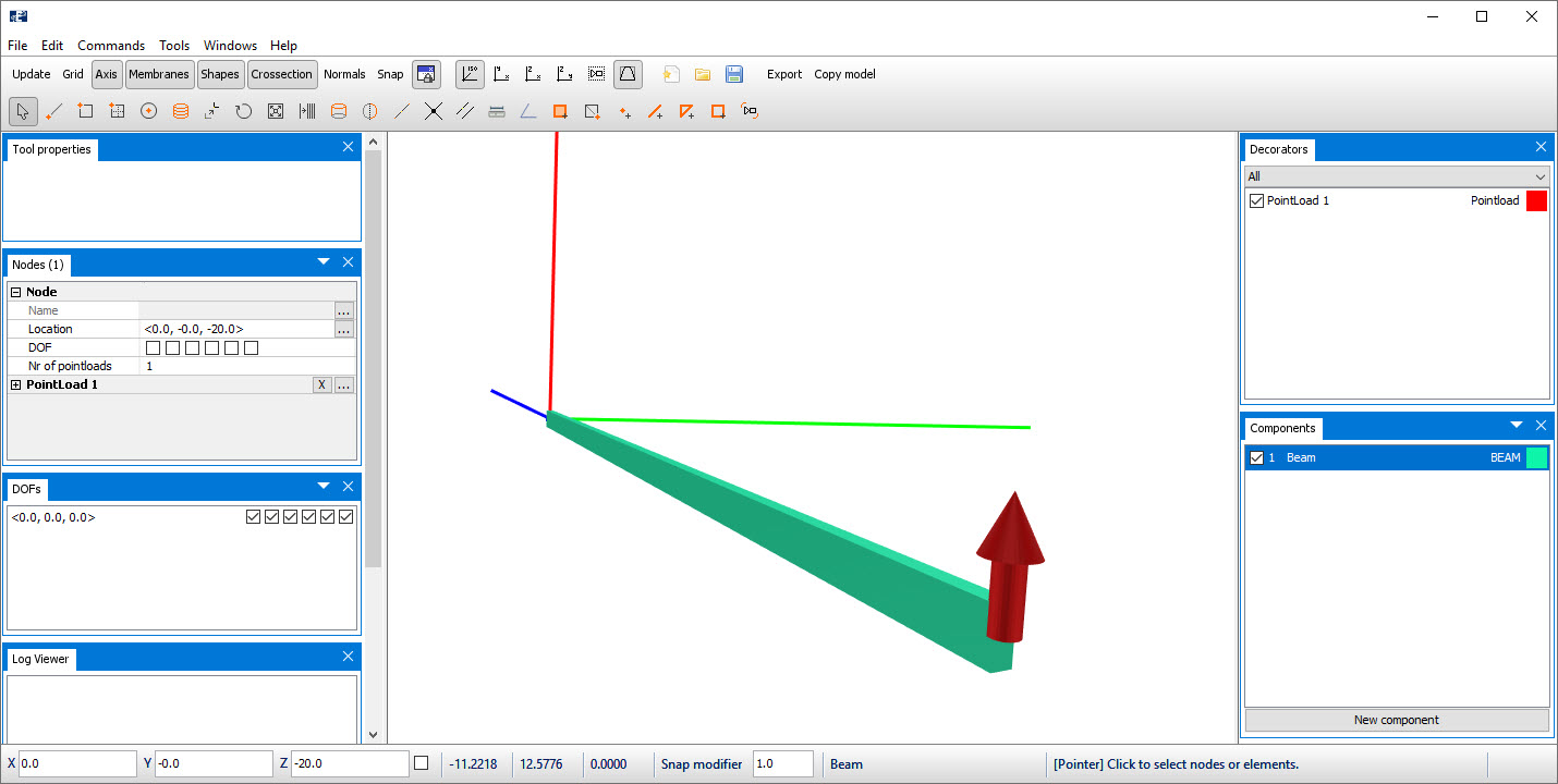
The model is now ready for analysis. Access the Environment window by selecting Export from the Toolbar. Leave the Time serie parameters and Export selections as described in section 2.4.

Export Selections

In the Environment window, select Export. Create a new folder for analysis. In this case study, we have created an analysis folder in Documents\AquaSim\Analyses\CaseStudy01 called Static02. Give the analysis a name e.g., static02_

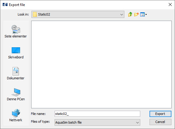
Select Export.

Run Analysis

The Analysis window appears. To start the analysis, press Start or Start all

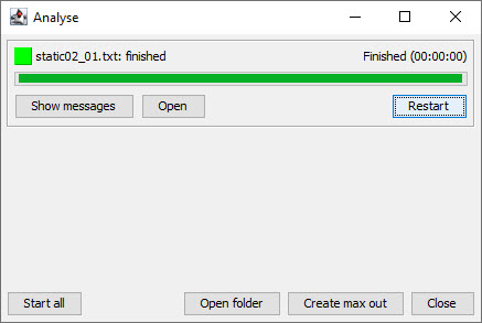
When the analysis changes the status from waiting to finished, select Open in the Analysis window. AquaView should be loaded.

Plot Shear Force

From the top Toolbar menu in AquaView, select Result > Local section forces > Shear force Z [N]. Jump to the last analysis step by selecting from the Playback control in the lower left corner of AquaView. Adjust the transparency of the water surface by dragging the blue bar in the top of the 3D view to the left.

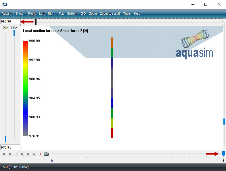
You may observe that the color of the beam is different for the first analysis.

Use your mouse pointer and right click on the free end of the beam in the 3D view. The Element result window will appear, presenting the results both as a table and a graph.

By selecting node B, the shear force for the free end is presented. Take note of the maximum value at node B is 996.99 N at step number 5

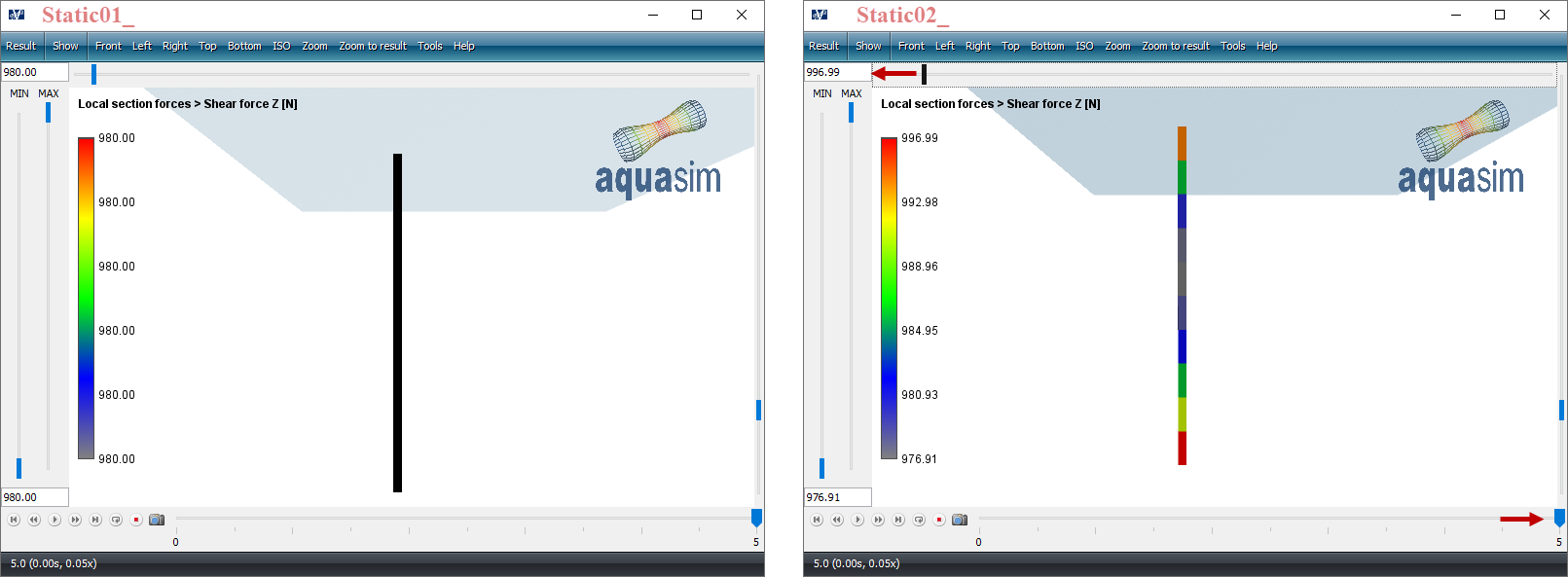
Comparing Results And Summary

By comparing the two analyses static01_ and static02_ it is seen that the discretization affects the results. Both color rendering and the magnitude of the shear force is affected

Model	Shear force Z [N]
1 element (Static01_)	980.0
10 elements (Static02_)	996.99

You can experience smaller differences between your own results, and the one presented here. This may be due to different solver versions being applied. We see that the shear force increases with more elements in the model. This is because the beam becomes less stiff with increased number of elements.

This case study is now finished