Analyses have been carried out for both regular- and irregular sea-states. Irregular waves are included to represent a realistic sea-condition. The controlled and repeatable nature of regular waves makes interpretation of results and comparison between analysis methods easier.

Results were evaluated by inspecting the overall cable response through the time-domain simulation, as well as by extracting timeseries and envelope results at selected locations along the cable. Figure 14 shows an example timestep an analysis with irregular waves.

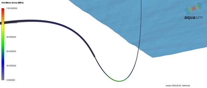
Figure 15 Timestep in simulation irregulars seas

A comparison study has been conducted, with the purpose of demonstrating that AquaSim predicts response and local cable behavior in line with established offshore analysis tools. The comparison focuses on key response quantities such as axial force, displacement and curvature. Regular sinusoidal waves are applied, with data as presented in section 6.1. The comparison is primary carried out in two ways:

• Comparison of maximum and minimum response values along the cable length:
  • Position 0 corresponds to the vessel attachment point,
  • Position 220 corresponds to the lower end node of the cable,
  • Most comparisons are limited to 200m, meaning 20 meters before the lower end node of the cable.
• Comparison of time series at selected cable locations.

Environmental data

The environmental data applied in the comparison is presented in Table 1. This represents a moderate sea state suitable for evaluating global and local response of the cable.

Table 1 Environmental data

Parameter	Value
Wave height [m]	4
Wave period [s]	8
Current velocity surface [m/s]	0.6
Current velocity z-exponent	7

Note that the current velocity decreases with depth. In AquaSim, this is represented through a depth-dependent current profile, defined by a table for varying current velocity with depth. This provides a more realistic representation of ocean current conditions compared with assuming a constant current velocity profile.

Time series parameters

Analyses with RAO-driven vessel motions may require a finer timestep discretization compared to analyses without vessel motion. The vessel response introduces additional dynamic excitation and higher-frequency response components that can be numerically sensitive. In this tutorial, a baseline timestep of 10ms has been applied. Too large timesteps may lead to inaccurate prediction of response amplitudes and loss of important dynamic behavior, as well as numerical instability.

Comparison of axial forces

Figure 16 and Figure 17 show comparison of maximum and minimum axial forces along the cable length. Axial force is one of the most important quantities for cable and riser systems, since it directly influences structural utilization and fatigue loading.

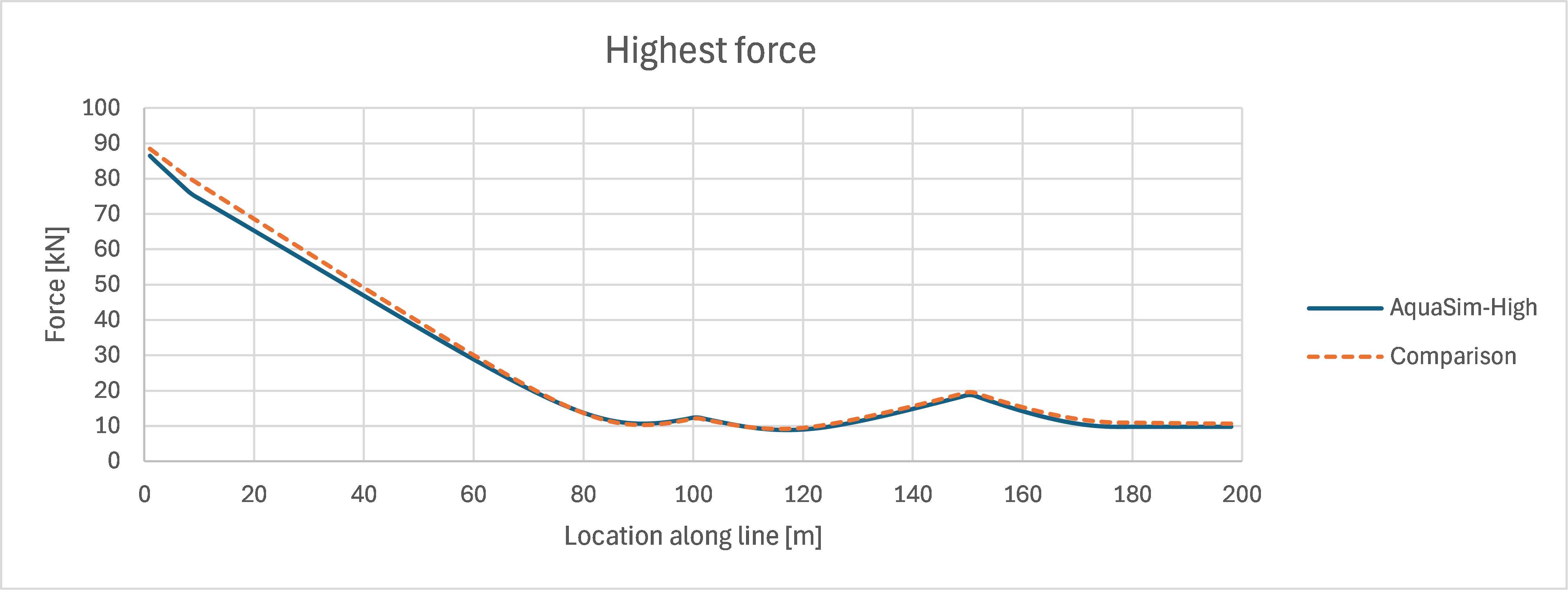
Figure 16 Max axial forces

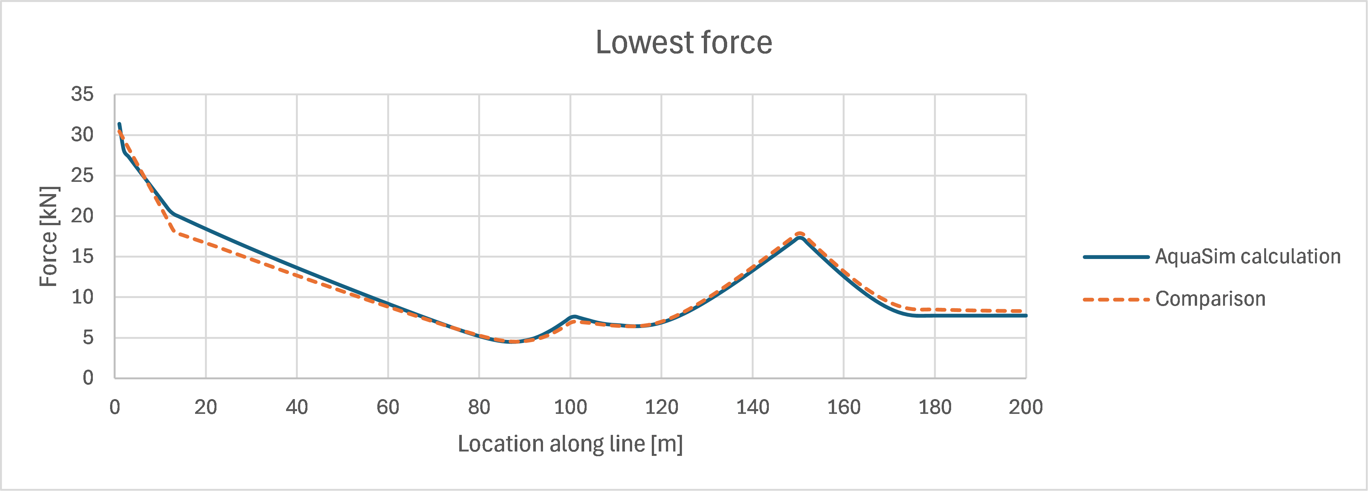
Figure 17 Min axial forces

As seen from Figure 16 and Figure 17, the results compare well through most parts of the cable length. The overall force distribution and response levels are consistent between AquaSim and the reference analysis.

Figure 18 presents the time series of axial force at the upper (*top) and lower (*end) end of the cable.

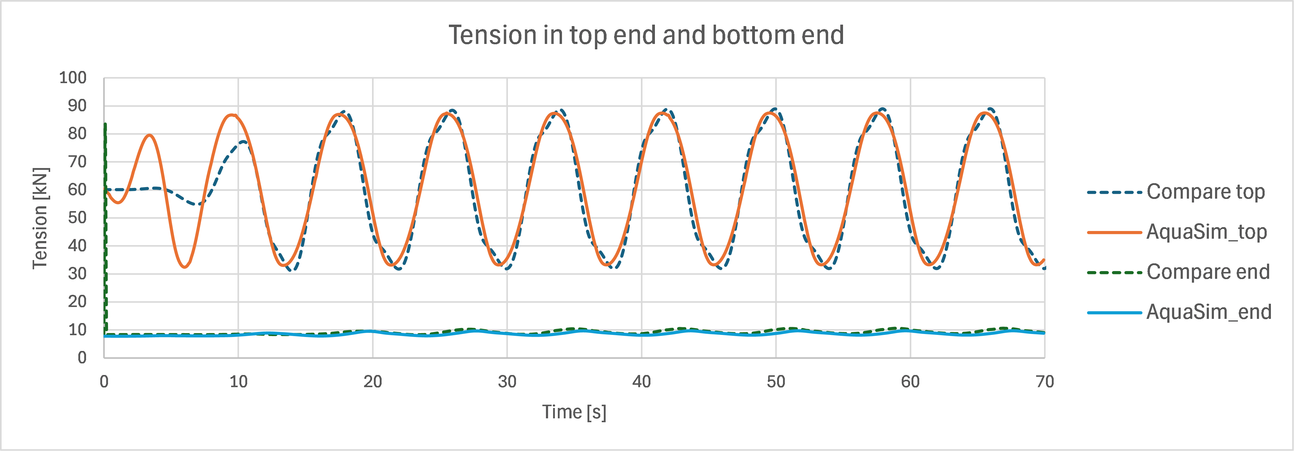
Figure 18 Time series axial forces at top node and end node

As seen from Figure 18, the results are in good agreement. The AquaSim time series is slightly smoother at the top node (vessel attachment node), where the reference results show minor deviations from a purely sinusoidal shape. These differences are small relative to the overall force magnitudes. A slight phase shift is observed at the lower node (back-end node), which is considered within acceptable engineering tolerances.

Figure 19 presents comparison of axial force (tensile) time series at locations 90m and 153m from the top node (vessel attachment node).

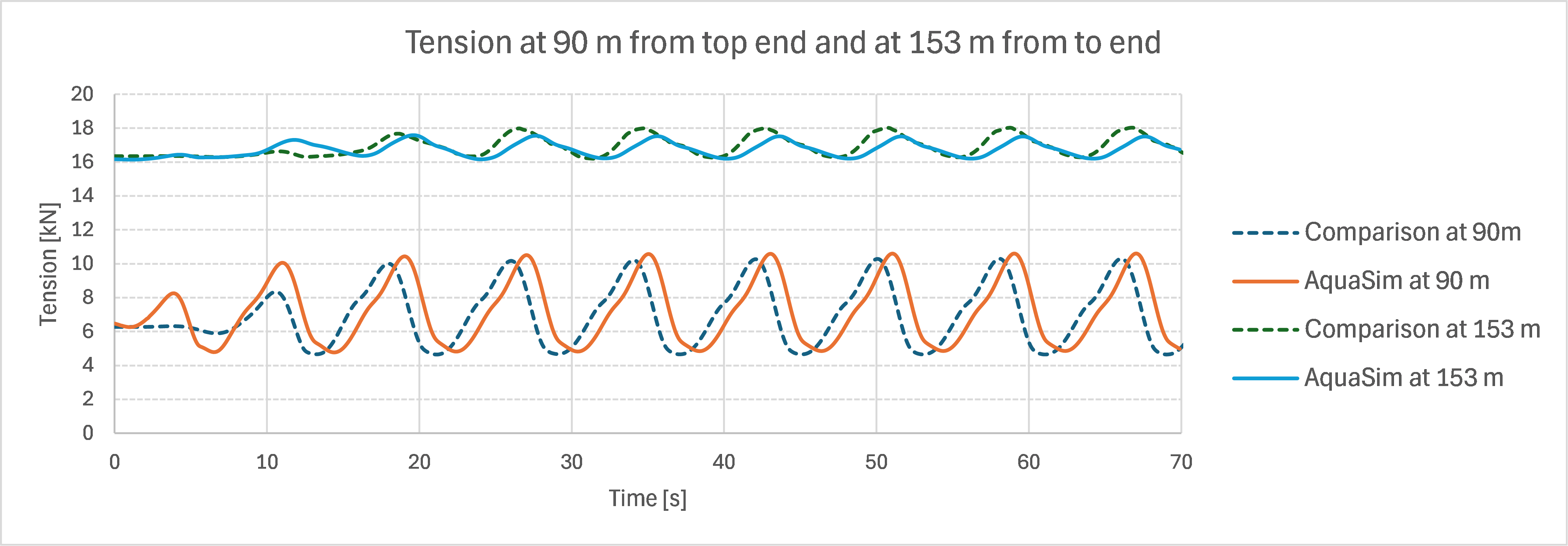
Figure 19 Time series axial forces at 90 m from top and 153 m from top.

These locations are selected in order to evaluate the response in different regions of the cable system, including both suspended and buoyancy-influenced sections. As seen from Figure 19, the results compare well. Minor differences in phase is observed, but the overall agreement is considered within acceptable limits.

Comparison of displacements

In Figure 20, the maximum vertical displacement along the cable is presented.

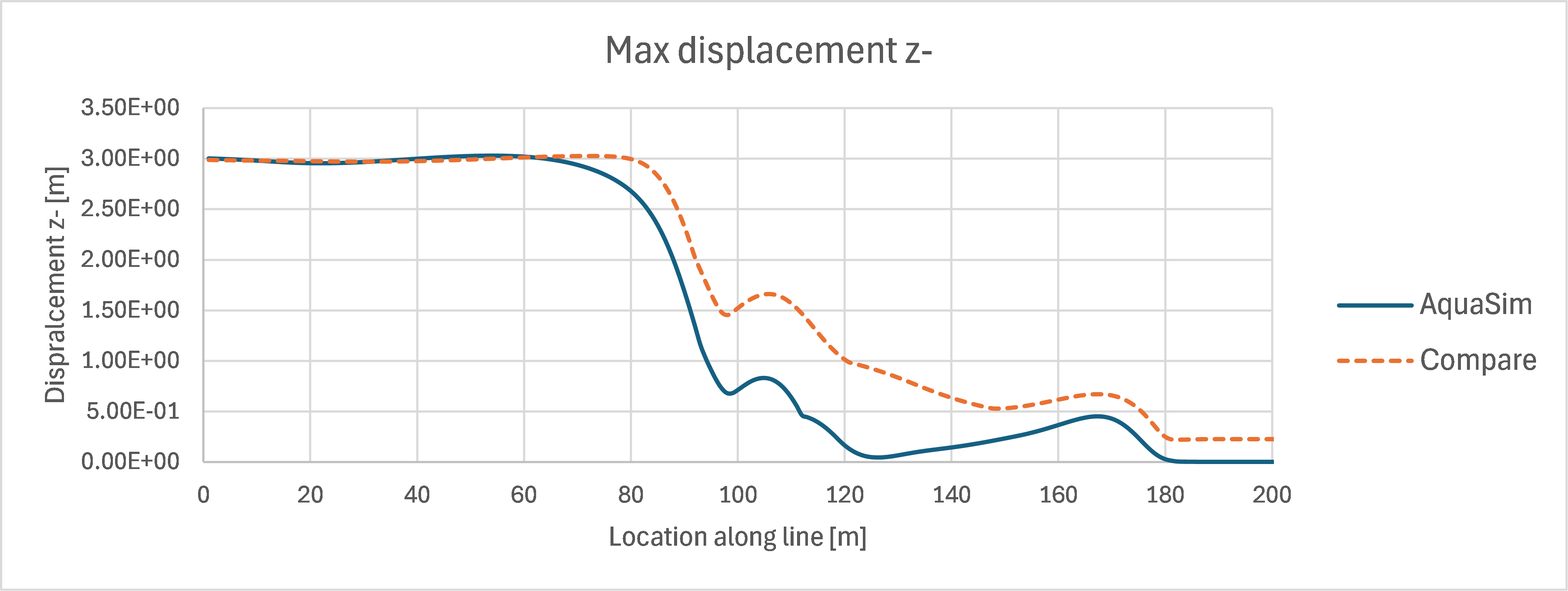
Figure 20 Max vertical displacement

Maximum vertical displacement shows close agreement in the upper part of the cable (i.e. from 0m to about 60m). Further down along the cable, AquaSim predicts somewhat lower vertical displacements compared to the reference analysis. The overall trend and shape of the displacement curve are nevertheless very similar. Which indicates that the global dynamic behavior, stiffness, hydrodynamic load and load transfer can be considered consistent between the two analysis tools. The remaining differences are relatively small and might be due to differences in timestep integration, local stiffness behavior or numerical damping formulation.

Comparison of curvature

Maximum curvature along the cable is presented in Figure 21. Curvature is relevant for evaluation of bending stresses and fatigue loading, since regions with high curvature are often associated with increased bending stresses and fatigue-related damage.

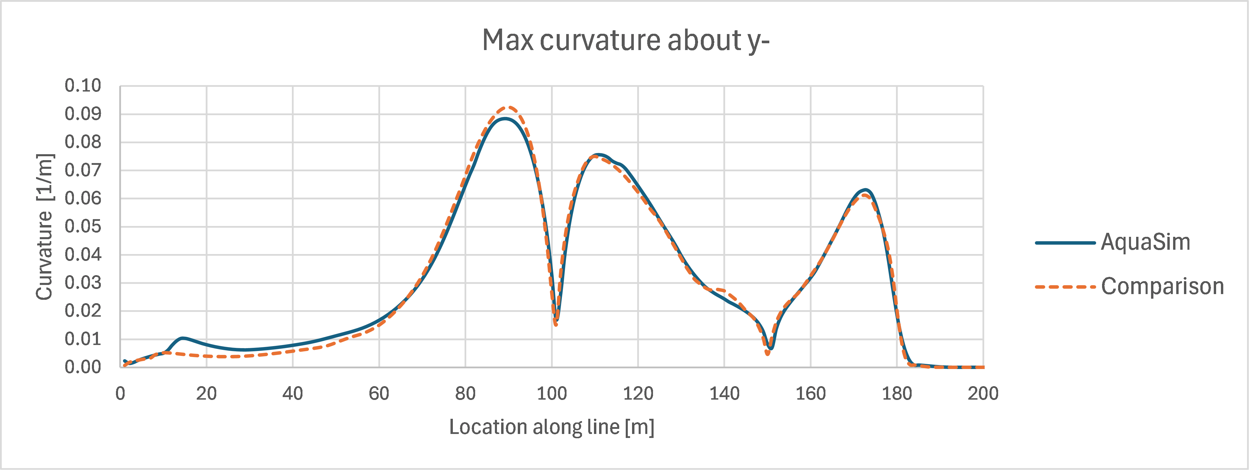
Figure 21 Max curvature in the analysis

The curvature in AquaSim compares well with the reference analysis throughout the cable length. The overall curvature distribution and peak regions are consistently predicted. In Figure 22, the curvature as a function of time is presented for two locations along the cable: at 90m from the vessel attachment node, and 153 m from the same reference point.

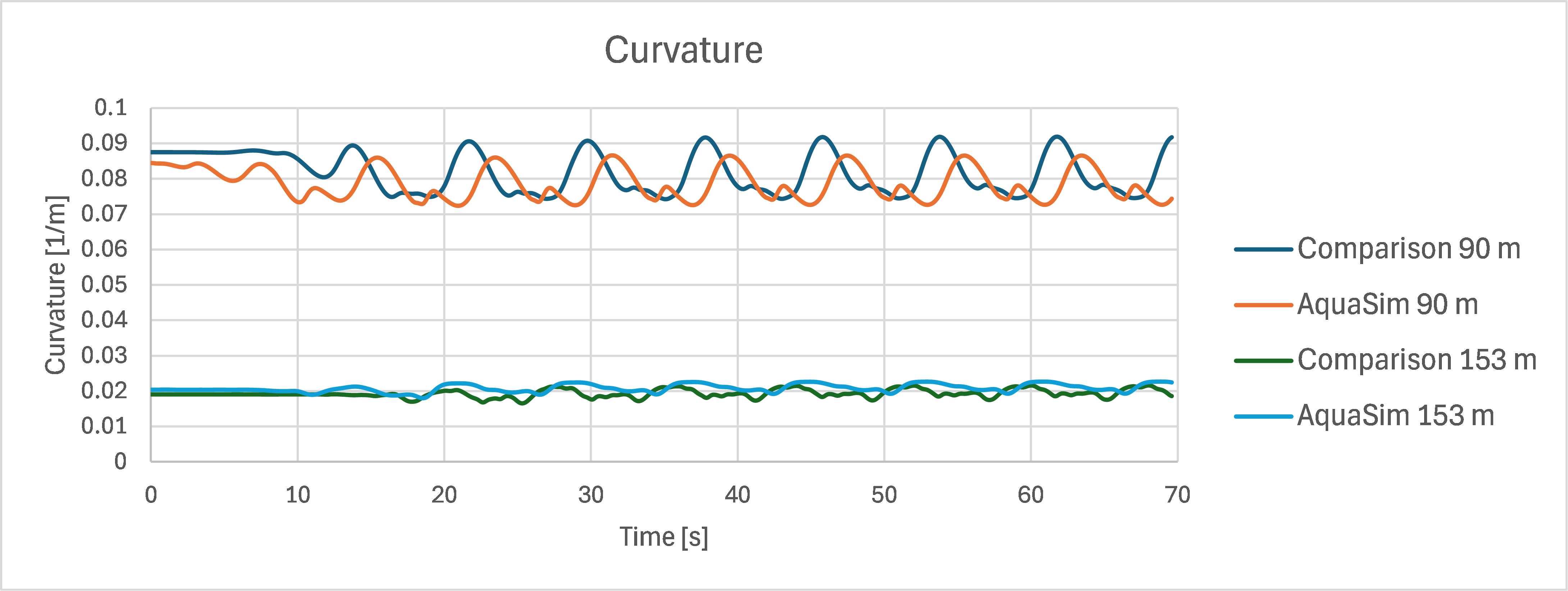
Figure 22 Curvature as function of time

As seen from Figure 22, the AquaSim curvature at 153m location is smoother than the reference analysis. At the 90m location, the dynamic variation about the equilibrium curvature shows a slightly smaller amplitude in AquaSim. Both observations are consistent with the slightly smoother dynamic response noted in the axial force comparison, and the overall agreement is considered satisfactory.