This section describes how to establish the numerical model in AquaEdit.

Stress-free condition

The cable is modelled in a stress-free condition, positioned along the global x-axis, 10 m above the mean water surface. This is illustrated in Figure 2. The cable is initially straight, without any tension or bending, and serves as the reference configuration before prescribed displacements, vessel motions, gravity, buoyancy and environmental loads are applied in the analysis.

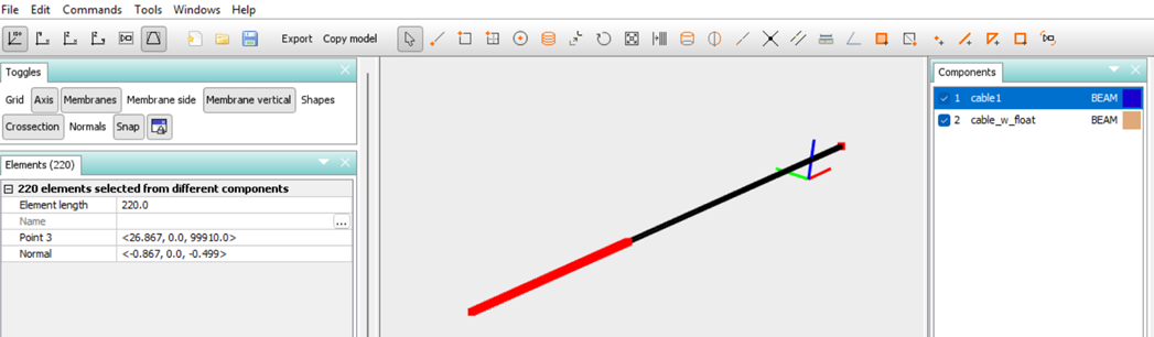Figure 2 Model of cable

Cable

The cable is modelled as Beam elements with bending stiffness. The total cable length is 220 m and is divided into two different components:

1. Cable: 170m without buoyancy segments,
2. Cable with buoyancy segments: 50m with buoyancy segments attached The two components are assigned different structural properties in order to represent the difference in mass, buoyancy, outer diameter, and hydrodynamic behavior.

Cable (without buoyancy segments)

The cable without buoyancy segments is modelled with the structural properties as illustrated in Figure 3. These properties define the axial stiffness, bending stiffness, mass and material characteristics of the cable. The hydrodynamic properties are given in Figure 4, which includes definition of how the cable should interact with the surrounding water, including drag and added mass effects.

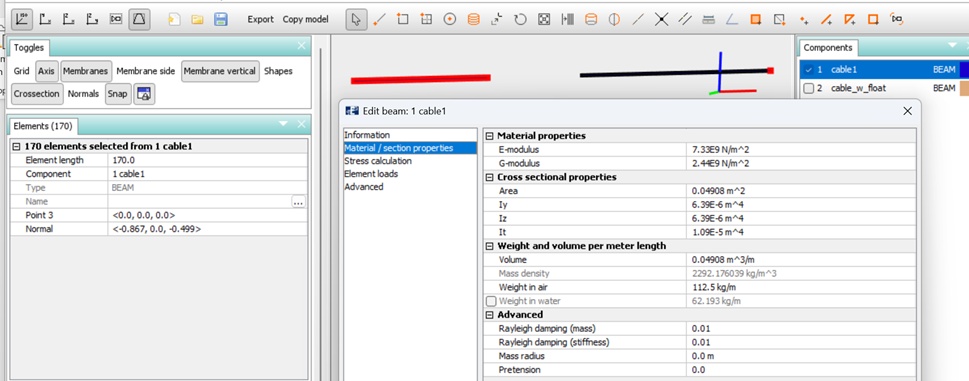Figure 3 Structural properties, part of cable without buoyancy segments

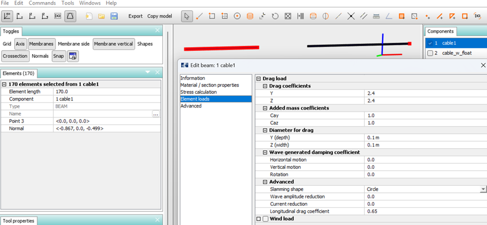Figure 4 Hydrodynamic properties cable without buoyancy segments

Cable with buoyancy segments

The cable section with buoyancy segments is modelled separately, with structural properties as provided in Figure 5. Compared to the bare cable section, this part has increased buoyancy and modified mass properties due to the attached floating segments. Hydrodynamic properties of the buoyancy segments are shown in Figure 6. The larger effective diameter and buoyancy will influence both the hydrodynamic loading and the response of the cable.

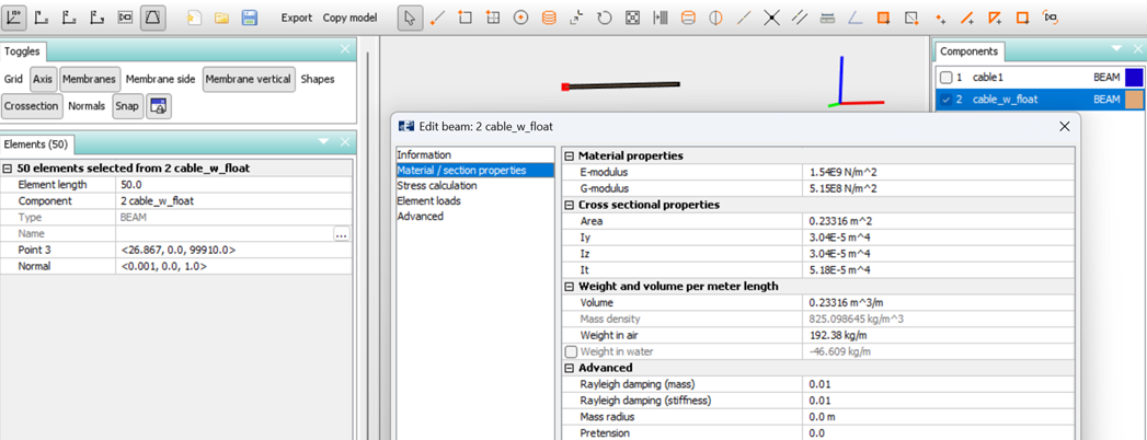Figure 5 Structural data, cable with buoyancy segments

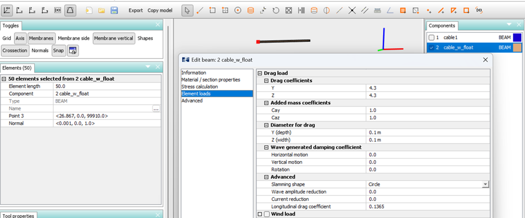Figure 6 Hydrodynamic properties, cable with buoyancy segments

Positioning of cable

As the cable system is modelled in a straight stress-free configuration, prescribed displacements and rotations are added in order to establish the desired installed geometry and pretension. This approach makes it possible to position the cable correctly before environmental loads are introduced.

Back-end node

Prescribed displacements are applied to the back-end node of the cable. The back-end node and its associated displacements are indicated in Figure 7.

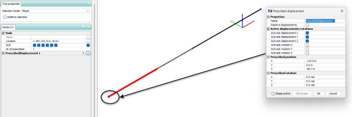Figure 7 Prescribed displacements to the back-end node of the cable

The following is established for the back-end node:'

• Prescribed displacements are applied only to the translatory DOFs,
• Rotational DOFs are left free, allowing the cable to rotate naturally and the back-end node,
• Prescribed position represents the assumed installation location of the cable end on the seabed.

The prescribed position should be verified through running a static equilibrium analysis. Small adjustments may be necessary to achieve the desired pretension and cable layout.

Attachment node on vessel

The upper end of the cable is connected to a vessel. In the present case study, vessel motions are represented by applying an RAO on this attachment node. Properties of this RAO is illustrated in Figure 8.

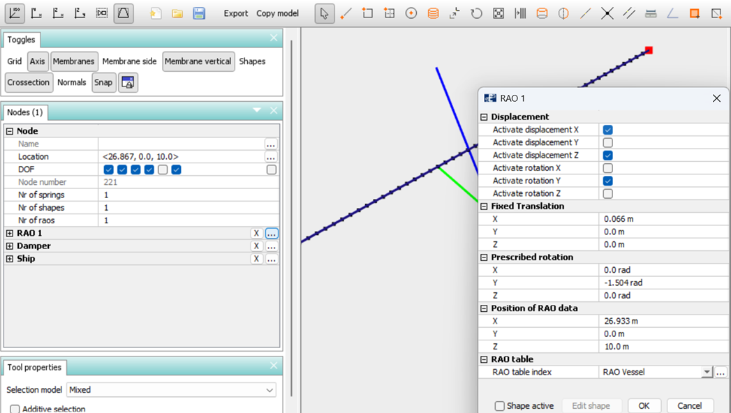Figure 8 RAO at vessel interface

The following is established for the RAO:

• RAO data is applied to translation in x- and z-direction, and rotation about y-axis,
• The node is assigned a fixed translation of 0.066m in x-direction,
• A prescribed rotation about the y-axis is applied to define the initial top angle of the cable. The prescribed rotational angle is close to 90degrees, consistent with the cable being modelled initially in a straight stress-free configuration,
• Position of the RAO table correspond to the x-position of the upper node connected to the vessel. It should be noted that the user must remember to activate the relevant DOFs in the Displacement section, in the upper part of the RAO dialogue.

Seabed contact

Contact between the cable and seabed is represented by assigning springs to nodes that may encounter the seabed. This is illustrated in Figure 9. 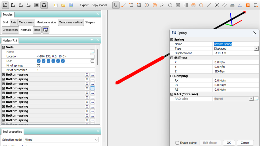Figure 9 Seabed interaction represented by springs of type Displacement

A total of 70 nodes is equipped with springs of type Displaced. The springs are activated when the nodal displacement exceeds the specified reference displacement. This reference displacement is established relative to the initial stress-free configuration of the model. Selection of spring stiffness may need to be tested and calibrated for individual cases:

• Too low stiffness may cause an unrealistic penetration of the seabed,
• Too high stiffness may cause increased convergence issues in the analysis.