Visual interpretation of results

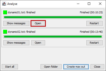
Load the result file from the first load condition by selecting Open from dynamic01.txt in the Analyse window.

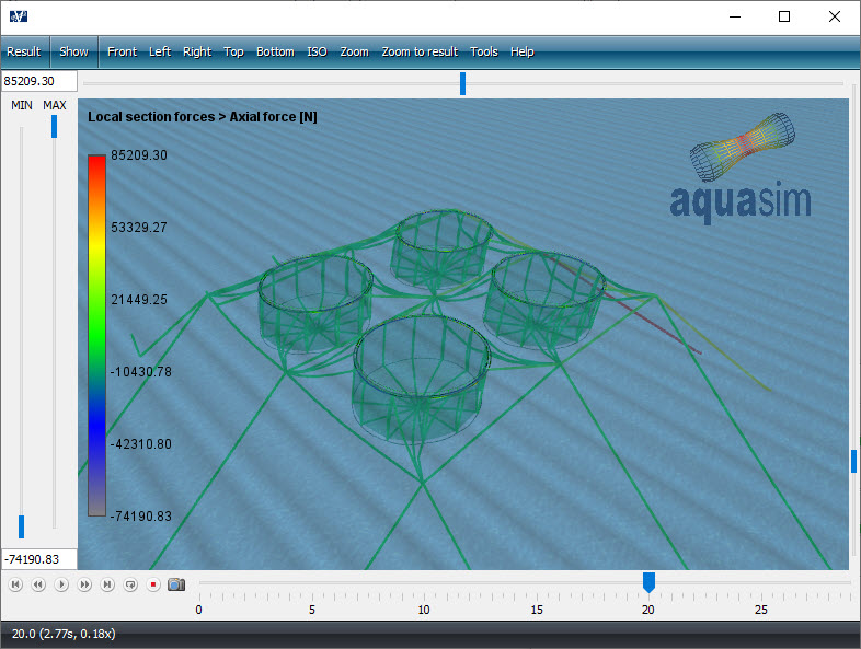
Load condition 01 will be loaded in AquaView. Plot Axial force [N] and play the analysis by selecting Play from the playback menu. Observe how the axial forces in the model evolve as waves and current passes the facility.

The playback speed can be adjusted by selecting Set duration from the playback menu. Unit is seconds, if you type 30 it will take 30 seconds to play from the first step to the last step.

When observing the analysis playback, you should observe the model behaving as expected. That is; forces in components rise when wave passes, the net deforms due to current and so on. This is a type of visual validation of the analysis. If you observe “jumping” elements or other abnormal response, this can indicate that the analysis has potential for improvements. An analysis can produce erroneous results despite achieved convergence for all steps. “Jumping” elements or other abnormal fluctuations may indicate a lack of damping in the system or eigen period issues. These considerations are not the scope of this case study but is highlighted as something to be aware of when working with dynamic problem solving.

Exit AquaView.

Load the result file from the second load condition by selecting Open from dynamic02.txt in the Analyse window.

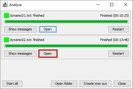
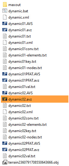
If you have closed the Analyse window, you may load the result file from your analysis folder in the File Explorer. Double click on dynamic02.avz.

In AquaView, you should plot the Axial force [N]. Follow the same procedure as for load condition 01, play the analysis and observe the response of your model. This is for visual validation of your model.

View terrain in AquaView

The terrain may be loaded in AquaView as well. In the Toolbar menu, select Show > Shapes > Terrain. Depth color can also be activated by selecting Toggle depth color in the Shapes menu. Adjust the transparency of the water surface by dragging the upper blue bar to the left.

Exit AquaView.

Maximum resulting forces

In this section you are to find maximum forces in the mooring components from the two analyzed load conditions. In your analysis folder, you will find a folder called maxout. Enter this folder. Here you will find files that contain maximum loads from both analyzes. These were generated when you selected Generate max out from the Analyse window in step number 32.

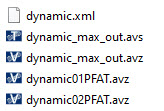
Load dynamic_max_out.avz by double click the file. AquaView will be loaded. If you failed to generate the maxout-files, you can find equivalent file in Documents\AquaSim\Demoes\CaseStudy03\Dynamic\maxout.

The maxout-file only contains maximum values from load condition 01 and 02, and consequently playback functionality is not available.

You should now find max axial force in the mooring components Frame rope (64mm), Bridle rope (48mm) and Mooring rope (64mm). From the Toolbar menu in AquaView, select Result > Local section forces > Max axial force [N].

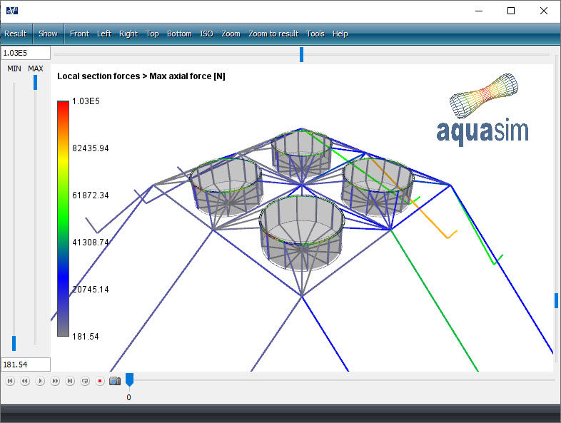
Press j on your keyboard to enter the window for maximum values of each component group.

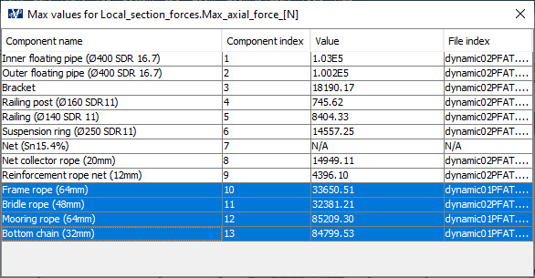
What the different columns in this window represent is provided in step number 29 in this case study. In addition, we have the column File index. This column indicates from which load condition the max values originate.

Copy the abovementioned components to clipboard by selecting component number 10 to 13 and CTRL + c. Paste the data in the same sheet you established from the static analysis.

Keep these figures for future reference when conducting CaseStudy04.

Dynamic considerations are now finished. Exit AquaView and AquaEdit.